Hands-On Tutorial Diffusion Models
In this tutorial, we are going to apply the theory Ito SDEs that we discussed in the last tutorial. We are going to implement the Ito SDE with affine drift coefficients to build a diffusion model and use it to sample from a simple distribution. Using a simple distribution allows to learn a lot about the inner workings of diffusion models, while still doing all the heavy lifting for implementing diffusion models for when we apply them to images. In the next tutorial, we are then going to apply these structures on images and scale it up.

import numpy as np
import matplotlib.pyplot as plt
from typing import Callable, List
from tqdm.notebook import tqdm
import matplotlib.pyplot as plt
import numpy as np
from IPython.display import HTML
import os
import torch
import torchvision
import torchvision.transforms as transforms
import torch.nn as nn
from torch.utils.data import Dataset
from torch import Tensor
from abc import ABC, abstractmethod
from torch.nn.functional import relu
from torch.utils.data.dataloader import DataLoader
from tqdm.notebook import tqdm
import scipy.stats as st

from utils import plot_2d_kde, plot_score_vector_field
1. Load Dataset
Let's build a very simple distribution in 2d that modulates a real-world scenario. Real-world data often lies on a manifold in a high-dimensional space (this is also called the Manifold hypothesis). For example, the set of all possible images does not cover any combination of pixel values but rather a subset that does cover full pixel space. We simulate such a scenario in 2d by making our data lie on a 1-dimensional manifold, i.e. a curve. We define a simple manifold defined by the quadratic function.
def manifold_func(x):
    return x**2

N_SAMPLES = 10000
x = torch.rand(size=(N_SAMPLES,))
y = manifold_func(x)
data = torch.stack([x,y],axis=1)

fig, ax = plt.subplots()
ax.scatter(data[:50,0],data[:50,1])
ax.set_xlim(-2,2)
ax.set_ylim(-2,2)
(-2.0, 2.0)
Let's define a simple pytorch dataset for it:
from torch.utils.data import Dataset, DataLoader
class ManifoldDataset(Dataset):
    def __init__(self, data: torch.Tensor):
        self.data = data

    def __len__(self):
        return len(self.data)

    def __getitem__(self, idx):
        data_item = data[idx]
        return data_item

dataset = ManifoldDataset(data)
batch_size = 128
trainloader = torch.utils.data.DataLoader(dataset, batch_size=batch_size, shuffle=True)
2. Define SDE
Next, we define an abstract class representation an Ito Stochastic Differental Equation: $$dX_t = f(X_t,t)dt + g(t)dW_t$$
The class requires you to specify:
-
cond_exp: the conditional expectation $\mathbb{E}[X_t|X_0]$ -
cond_var: the conditional variance $\mathbb{V}[X_t|X_0]$ -
f_drift: the drift function $f:\mathbb{R}^d\times\mathbb{R}\to\mathbb{R}^d$. -
g_random: the infinitesimal variance $g:\mathbb{R}\to\mathbb{R}$.
Moreover, it has functions that evolve the SDE forward and backward. We assume throughout this chapter that conditional expectations and variances $\mathbb{E}[X_t|X_0], \mathbb{V}[X_t|X_0]$ can be analytically computed and that conditional distributions are Gaussian. This is in particular true for ItoSDEs for affine drift coefficients as we have seen.
class ItoSDE(ABC):
    def __init__(self, T_max: float):
        self.T_max = T_max

    @abstractmethod
    def cond_exp(self, X_0: Tensor, t: Tensor):
        pass

    @abstractmethod
    def cond_var(self, X_0: Tensor, t: Tensor):
        pass

    @abstractmethod
    def f_drift(self, X_t: Tensor, t: Tensor):
        pass

    @abstractmethod
    def g_random(self, X_t: Tensor, t: Tensor):
        pass

    def cond_std(self, X_0: Tensor, t: Tensor):
        """Conditional standard deviation. Square root of self.cond_var."""
        return torch.sqrt(self.cond_var(X_0=X_0,t=t))

    def sample_random_times(self, length: int):
        """Sample 'length' time points uniformly in interval [0,T]"""
        return torch.rand(size=(length,))*self.T_max

    @staticmethod
    def _mult_first_dim(t,X):
        """
        Helper function to multiply one-dimensional time vector with tensor of
        arbitrary shape.
        Inputs:
            X_0: shape (n,*,*,...,*)
            t: shape (n)
        Outputs:
            has same shape as X_0 - inputs X_0[i] multipled with t[i]
        """
        return t.view(-1,*[1]*(X.dim()-1))*X

    def run_forward(self, X_0: Tensor, t: Tensor, clip_factor: float = 0.01):
        """
        Function to evolve SDE forward in time from 0 to t<=self.T_max.
        Assume that conditional distribution is Gaussian
        Inputs:
            X_0: shape (n,*,*,...,*)
            t: shape (n)
        Outputs:
            X_t: shape as X_0 - noised input
            noise: shape as X_0 - noise converting X_0 to X_t
            score: shape as X_0 - score of conditional distribution q_t|0(X_t|X_0)
        """
        noise = torch.randn(size=X_0.shape)
        cond_std = self.cond_std(X_0,t)
        cond_exp = self.cond_exp(X_0,t)
        X_t = self._mult_first_dim(cond_std,noise)+cond_exp
        if clip_factor is not None:
            cond_std = torch.clip(cond_std,min=clip_factor)
        score = -self._mult_first_dim(1/cond_std,noise)

        return X_t, noise, score

    def run_forward_random_times(self, X_0: Tensor):
        """Function to evolve SDE forward until random times."""
        t = self.sample_random_times(X_0.shape[0])
        X_t, noise, score = self.run_forward(X_0,t)
        return X_t, noise, score, t
2.1 Variance-preserving SDE
Let's implement the variance-preserving SDE that is the basis for the first formulation of diffusion models with:
- $f(x,t)=-\frac{1}{2}x\beta'(t)$
- $g=\sqrt{\beta'(t)}$
- $\beta(t)=t\beta_{\text{min}}+\frac{1}{2}t^2(\beta_{\text{max}}-\beta_{\text{min}})$
- $\beta'(t)=\beta_{\text{min}}+t(\beta_{\text{max}}-\beta_{\text{min}})$
- $\mathbb{E}[X_t|X_0] = \exp(-0.5\beta(t))$
- $\mathbb{V}[X_t|X_0] = 1-\exp(\beta(t))$
I.e. the expectation exponentially decays to $0$ while the conditional variance converges to one - the variance $\mathbb{V}[X_t]=1$ if we assume that the data is normalized to variance 1 (see the last tutorial for an explanation and derivation).
class VPSDE(ItoSDE):
    def __init__(self,T_max: float, beta_min: float = 0.0, beta_max: float = 1.0):
       self.T_max = T_max
       self.beta_min = beta_min
       self.beta_max = beta_max

    def _beta_derivative(self, t: Tensor):
        return self.beta_min+(self.beta_max - self.beta_min)*t

    def _beta(self, t: Tensor):
        return (self.beta_min*t)+0.5*(self.beta_max - self.beta_min)*(t**2)

    def cond_exp(self, X_0: Tensor, t: Tensor):
        """
        Inputs:
            X_0: shape (n,*,*,...,*)
            t: shape (n)
        Outputs:

        """
        assert len(t.shape) == 1, "Time must be 1-dimensional."
        assert t.shape[0] == X_0.shape[0]
        beta_t = self._beta(t)
        cond_exp_t = torch.exp(-0.5*beta_t)
        return self._mult_first_dim(cond_exp_t,X_0)

    def cond_var(self, X_0: Tensor, t: Tensor):
        """
        Inputs:
            X_0: shape (n,*,*,...,*)
            t: shape (n)
        Outputs:

        """
        assert len(t.shape) == 1, "Time must be 1-dimensional."
        #assert t.shape[0] == X_0.shape[0]
        beta_t = self._beta(t)
        cond_var_t = 1-torch.exp(-beta_t)
        return cond_var_t


    def f_drift(self, X_t: Tensor, t: Tensor):
        """
        Inputs:
            X_0: shape (n,*,*,...,*)
            t: shape (n)
        Outputs:

        """
        assert len(t.shape) == 1, "Time must be 1-dimensional."
        assert t.shape[0] == X_t.shape[0]
        deriv_beta_t = self._beta_derivative(t)
        return -0.5*self._mult_first_dim(deriv_beta_t,X_t)

    def g_random(self, t: Tensor):
        """
        Inputs:
            X_0: shape (n,*,*,...,*)
            t: shape (n)
        Outputs:

        """
        assert len(t.shape) == 1, "Time must be 1-dimensional."
        deriv_beta_t = self._beta_derivative(t)
        return torch.sqrt(deriv_beta_t)
Let's define an example SDE:
sde = VPSDE(T_max=1,beta_min=0.01, beta_max=2.0)
Let's plot the forward-evolution from $t=0$ (original distribution) to $t=1$ (Gaussian noise). It nicely converges towards Gaussian noise.
n_grid_points = 8
time_vec = torch.linspace(0,1,n_grid_points)**2
X_0 = torch.stack([torch.stack([dataset.__getitem__(idx)]*n_grid_points) for idx in range(1000)]).transpose(1,0)
X_t, noise, score = sde.run_forward(X_0,time_vec)

fig, axs = plt.subplots(1,n_grid_points, figsize=(6*n_grid_points,6))
for idx in range(n_grid_points):
    axs[idx].scatter(X_t[idx,:,0],X_t[idx,:,1])
    axs[idx].set_xlim(-1.5,1.5)
    axs[idx].set_ylim(-1.5,1.5)
    axs[idx].set_title(f"time step = {time_vec[idx]:.2f}")
3. Neural network
Next, we define the neural network that we need to train. As we have seen in the last tutorial, there are two options: we can either train a neural network $s_{\theta}(x_t,t)$ to approximate a score $\nabla_{x_t} \log p_t(x_t|x_0)$ or we can train a neural network $\epsilon_{\theta}(x_t,t)$ to predict the noise an image has been distored. Both cases are related:
$$ \begin{align*}&\epsilon_{\theta}(x_t,t)=-s_{\theta}(x_t,t)\sqrt{\mathbb{V}[X_t|X_0=x_0]}\\ \Leftrightarrow &s_{\theta}(x_t,t)=-\frac{\epsilon_\theta(x_t,t)}{\sqrt{\mathbb{V}[X_t|X_0=x_0]}}\end{align*}$$
where $\mathbb{V}[X_t|X_0]=1-\exp(-\beta(t))$.
I introduce a flag TRAIN_SCORE that you can set to switch between both options. Consistent with literature, I found that training the denoising network leads to more stable training and therefore we train a neural network $\epsilon_{\theta}(x_t,t)$ but feel free it.
TRAIN_SCORE = False #whether to train score or denoiser network
As a neural network, I simply use a fully connected neural network that conatenates $x$ and $t$.
import torch
import torch.nn as nn
import torch.nn.functional as F

class FullConnectedScoreModel(nn.Module):
    def __init__(self, data_dim: int = 2, hidden_dim: int = 128, n_hidden_layers: int = 2):
        super(FullConnectedScoreModel, self).__init__()

        # Input layer
        self.input_layer = nn.Linear(data_dim+1, hidden_dim)
        self.input_batch_norm = nn.BatchNorm1d(hidden_dim)

        # Hidden layers
        self.hidden_layers = nn.ModuleList()
        for _ in range(n_hidden_layers):
            layer = nn.Linear(hidden_dim, hidden_dim)
            batch_norm = nn.BatchNorm1d(hidden_dim)
            self.hidden_layers.append(nn.Sequential(layer, batch_norm))

        # Output layer
        self.output_layer = nn.Linear(hidden_dim, data_dim)  # Assuming output is a single value

    def forward(self, x, t):
        x_conc_t = torch.concat([x,t.unsqueeze(1)],axis=1)
        x = F.relu(self.input_batch_norm(self.input_layer(x_conc_t)))

        for hidden_layer in self.hidden_layers:
            x = F.relu(hidden_layer(x))

        return self.output_layer(x)
model = FullConnectedScoreModel()
Let's initialize the training parameters:
LEARNING_RATE = 2e-5
WEIGHT_DECAY = 1e-5
N_EPOCHS = 10

optimizer = torch.optim.Adam(model.parameters(),lr=LEARNING_RATE, weight_decay=WEIGHT_DECAY,maximize=False)
device = "cuda" if torch.cuda.is_available() else "cpu"
We can now define the function that trains the neural network, i.e. minimizes the loss:
\begin{align*} L(\theta) &=\mathbb{E}_{t\sim\text{Unif}_{[0,T]}}\left[\mathbb{E}_{x_0\sim p_{\text{data}}}\mathbb{E}_{\epsilon\sim\mathcal{N}(0,\mathbb{1})}\left[\|\epsilon_{\theta}(\sqrt{\mathbb{V}[X_t|X_0=x_0]}\epsilon+\mathbb{E}[X_t|X_0=x_0],t)-\epsilon\|^2\right]\\\right] \end{align*}
def train_diffusion_model(model, sde: ItoSDE, dataloader: DataLoader, optimizer, device, n_epochs: int, print_every: int, train_score: bool = TRAIN_SCORE):
    model.train()
    model = model.to(device)
    loss_function = nn.MSELoss(reduction='mean')
    running_loss_list = []

    for epoch in range(n_epochs):
        print(f"Epoch: {epoch}")
        running_loss = 0.0
        for idx, x_inp in enumerate(dataloader):

            #Zero gradients:
            optimizer.zero_grad()

            #Run forward samples:
            X_t,noise,score,time = sde.run_forward_random_times(x_inp)

            #Send to device:
            X_t = X_t.to(device)
            noise = noise.to(device)
            time = time.to(device)

            #Predict score:
            model_pred = model(X_t,time)

            #Compute loss:
            if train_score:
                loss = loss_function(score,model_pred)
            else:
                loss = loss_function(noise,model_pred)

            #Optimize:
            loss.backward()
            optimizer.step()

            # print statistics
            running_loss += loss.detach().item()

            if (idx+1) % print_every == 0:
                avg_loss = running_loss/print_every
                running_loss_list.append(avg_loss)
                running_loss = 0.0
                print(avg_loss)
    return model,running_loss_list
model,running_loss_list = train_diffusion_model(model, sde, trainloader, optimizer, device=device, n_epochs=N_EPOCHS, print_every=10)
Epoch: 0
1.107963615655899
1.0125799179077148
0.9075559198856353
0.7546133399009705
0.6844007015228272
0.6064333200454712
0.589002525806427
Epoch: 1
0.49831153452396393
0.4876184225082397
0.4710222542285919
0.4200606018304825
0.396854630112648
0.3988864660263062
0.4038829684257507
Epoch: 2
0.39687347412109375
0.33917929530143737
0.35203162431716917
0.3338125616312027
0.3114520773291588
0.3419607937335968
0.3362072065472603
Epoch: 3
0.30856805443763735
0.32144091129302976
0.3035150021314621
0.3088932827115059
0.3109659790992737
0.32022510319948194
0.3144350528717041
Epoch: 4
0.31018681824207306
0.2929459050297737
0.3099128261208534
0.3085441797971725
0.2968200445175171
0.26700222939252855
0.2981332078576088
Epoch: 5
0.30222111344337466
0.26633969992399215
0.30578442513942716
0.2757169172167778
0.2628078654408455
0.27507842630147933
0.2782664254307747
Epoch: 6
0.2716243967413902
0.2923890143632889
0.2789475813508034
0.2826638177037239
0.25543404519557955
0.2546220481395721
0.2774943709373474
Epoch: 7
0.2634443029761314
0.26807230710983276
0.28426249623298644
0.251651032269001
0.28233994394540785
0.26316439509391787
0.28055903166532514
Epoch: 8
0.2576915830373764
0.26831352561712263
0.2831210345029831
0.2793415397405624
0.24959432184696198
0.2650570452213287
0.2619884729385376
Epoch: 9
0.2780921012163162
0.24066464602947235
0.2636589199304581
0.2784975990653038
0.25768794268369677
0.2597701773047447
0.29261800944805144
model = model.to("cpu")
Let's plot the score vector field $\nabla_{x_t}\log p_t(x_t) = \epsilon_{\theta}(x_t,t)/\sqrt{(1-\exp(-\beta(t)))}$ that we have learnt. We can see that the score vector field pushes the data points to the data manifold over time:
plot_score_vector_field(model,t=1.0,min_x=-2.0,max_x=2.0, sde=sde, train_score=TRAIN_SCORE)
plot_score_vector_field(model,t=0.5,min_x=-2.0,max_x=2.0, sde=sde, train_score=TRAIN_SCORE)
plot_score_vector_field(model,t=0.25,min_x=-2.0,max_x=2.0, sde=sde, train_score=TRAIN_SCORE)
plot_score_vector_field(model,t=0.0,min_x=-2.0,max_x=2.0, sde=sde, train_score=TRAIN_SCORE)
<Axes: >
5. Model deployment
Finally, let's run SDE backwards with the equation that we derived: $$\begin{align*}&d\bar{X}_t= [f(X_t,t)-g^2(t)s_{\theta}(x,t)dt + g(t)d\bar{W}_t\\ \Leftrightarrow& \bar{X}_{t-s} \approx \bar{X}_t -s\left[g^2(t)\frac{\epsilon_{\theta}(\bar{X}_t,t)}{\sqrt{1-\exp(-\beta(t))}}+f(\bar{X}_t,t)\right]+\sqrt{s}g(t)\epsilon \quad \text{ where } \epsilon\sim\mathcal{N}(0,I)\end{align*}$$
where we clip the denominator $\sqrt{1-\exp(-\beta(t))}$ to avoid numerical instability when the denonimator is close to zero:
def run_backwards(model: torch.nn.Module, sde: ItoSDE, x_start: Tensor, device, train_score, n_steps: int = 10, plot_evolution: bool = True, clip_max: float = 1.0, clip_min: float = -1.0, **kwargs):
    """Function to run stochastic differential equation. We assume a deterministic initial distribution p_0."""
    model = model.to(device)

    #Number of trajectories, dimension of data:
    n_traj = x_start.shape[0]
    ndim = x_start.dim()-1

    #Compute time grid for discretization and step size:
    time_grid = torch.linspace(sde.T_max,0,n_steps)
    step_size =torch.abs(time_grid[0]-time_grid[1])

    #Compute the random drift at every time point:
    random_drift_grid = sde.g_random(time_grid)

    #Sample random drift at every time point:
    noise = torch.randn(size=(n_steps,*list(x_start.shape)))
    random_drift_grid_sample = torch.sqrt(step_size) * noise * random_drift_grid.view(-1,*[1]*(ndim+1))

    #Initialize list of trajectory:
    x_traj = [x_start]

    if plot_evolution:
        fig, axs = plt.subplots(1,len(time_grid),figsize=(6*len(time_grid),6))


    for idx,time in tqdm(enumerate(time_grid)):

        #Get last location and time
        x = x_traj[idx]
        t = time_grid[idx]
        time_vec = t.repeat(n_traj)

        #Deterministic drift: f(X_,t)
        determ_drift = step_size*sde.f_drift(x,time_vec)

        #Get random drift:
        random_drift_sample = random_drift_grid_sample[idx]

        #Get noise estimates:
        model_estimate = model(x.to(device),time_vec.to(device)).detach().cpu()

        if train_score:
            score_estimates = model_estimate
        else:
            denominator = torch.clip(sde.cond_std(None, time_vec),0.01)
            if len(model_estimate.shape) == 4:
                score_estimates = -model_estimate/denominator[:,None,None,None]
            else:
                score_estimates = -model_estimate/denominator[:,None]

        #Correction term: g^2 * score estimate
        g_squared = (random_drift_grid[idx]**2).repeat(n_traj)
        correction_term = (step_size*ItoSDE._mult_first_dim(g_squared,score_estimates))

        #Compute next step:
        change = (correction_term - determ_drift) + random_drift_sample
        next_step = x + change

        #Save step:
        x_traj.append(next_step)

        if plot_evolution:
            axs[idx].scatter(next_step[:,0],next_step[:,1])
            axs[idx].quiver(next_step[:,0],next_step[:,1],change[:,0],change[:,1])
            axs[idx].set_xlim(-2.0,2.0)
            axs[idx].set_ylim(-2.0,2.0)
            axs[idx].set_title(f"Step={idx}")

    output = torch.stack(x_traj) #.transpose(1,0)
    #output = torch.clip(output, clip_min, clip_max)
    return output,time_grid
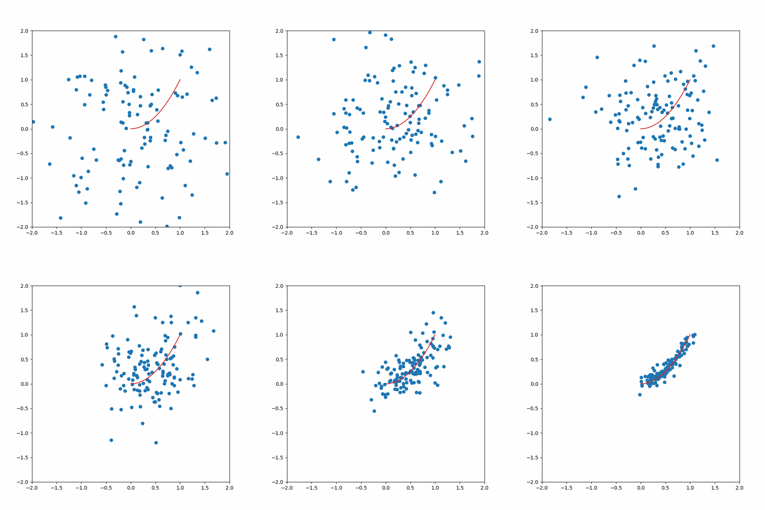
Let's randomly sample and plot the vectors pushing the data points to the manifold:
x_start = torch.randn(size=next(enumerate(trainloader))[1].shape)
output,time_grid = run_backwards(model,sde,x_start=x_start,n_steps=10,device=device, train_score=TRAIN_SCORE)
0it [00:00, ?it/s]
And let's finally plot the distribution over time:
from celluloid import Camera # getting the camera
import matplotlib.pyplot as plt
import numpy as np
from IPython.display import HTML # to show the animation in Jupyter
# the camera gets the fig we'll plot

fig, axs = plt.subplots(figsize=(7,7))
camera = Camera(fig)
x_ref = np.linspace(0,1,100)
for idx in range(output.shape[0]):
    axs.plot(x_ref, manifold_func(x_ref),color='tab:red')
    axs.scatter(output[idx,:,0],output[idx,:,1],color='tab:blue')
    axs.set_xlim(-2.0,2.0)
    axs.set_ylim(-2.0,2.0)
    camera.snap()

animation = camera.animate() # animation ready
animation.save('diffusion_model_sampling.gif')
plt.close()
MovieWriter ffmpeg unavailable; using Pillow instead.
from IPython.display import HTML
HTML('<img src="diffusion_model_sampling.gif"">')

6. Conclusion
We trained our first diffusion model with SDEs! As a next step, we are going to use the above implementation on images.